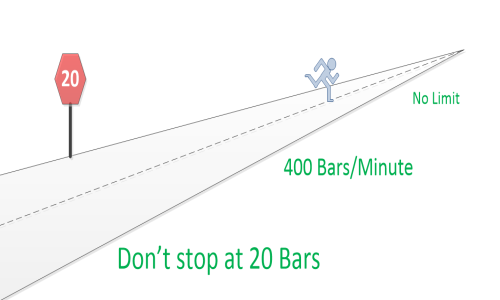
Faster Many orders of magnitude faster
Speed changes everything
- Faster solver - 400 Bars/min
- Scales linearly - Very complex risk models doable
- Quant model sample size independent
- Patents issued and pending
A new method to solve Risk-Reward problems.
Solves faster - with full accuracy across the entire span of every probability distribution calculated.
Scales linearly with number of models used.
This means
very complex risk models are now doable.
Traditional (
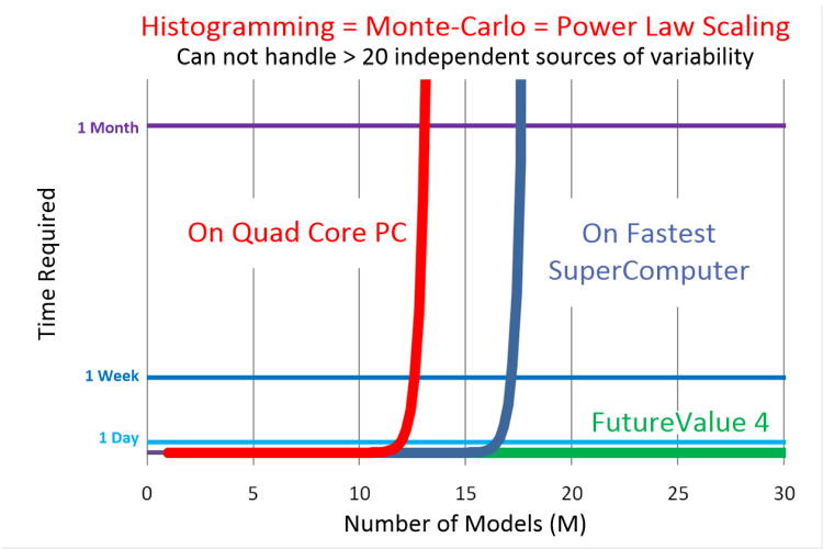
Monte-Carlo - histogramming) modeling has Power Law scaling.
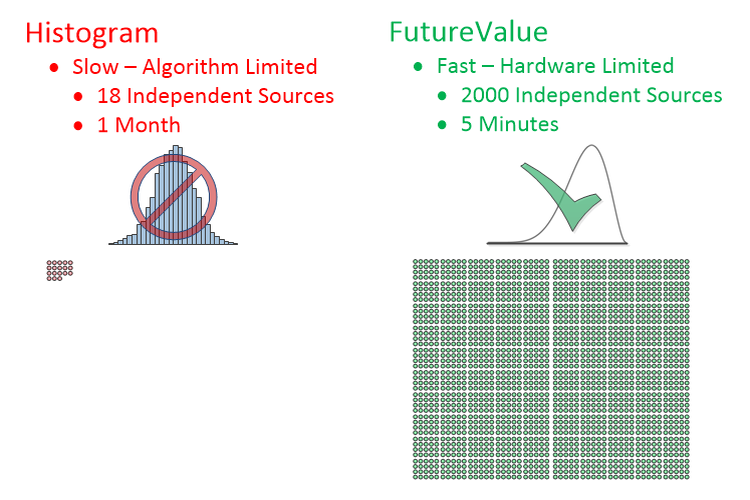
Aggregation through histogramming can not handle > 20 independent models.
Could use your existing quant models as inputs. Removes many of the limits binding current Risk-Reward modeling
Details
So, you have a bunch of quantitative finance models. That's not where
your problem lies.
The problem with traditional financial modeling lies in trying to combine
them into an aggregate result.
Note: We can use your quant models as input into our methods, and get
around the limitations your traditional methods have on the number of independent
sources of variability.
Although, they take a lot to develop and prove out, and we think we've
got a
better way.
Traditional methods = slow & limited:
The speed problem lies in trying to combine various models to predict
outcomes for a portfolio. The traditional way to do this is by using
Monte-Carlo methods.:
- Performing many runs of various models that each produce single values - scalar models
- Asigning likelihood to each model's scalar result
- Aggregating the results from the various scalar models by combining their values and likelihoods
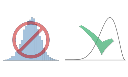
- Binning the result in a histogram of aggregate value vs. likelihood
- Often - fitting some continuous probability distribution to the histogram - claiming the distribution fits the data
Basically, each model produces a single point solution, and you combine solutions from each model to get an aggregate liklihood for one set of conditions. Do this many times - for different conditions. Then, histogram the results to approximate a probability distribution at some point in time. By example, and oversimplifying, think of Monte-Carlo method as playing Yahtzee with 5 crooked dice. By throwing them often enough, and adding the scores, you can estimate the most likely aggregate outcome.
The fewer times you throw the dice (sample your models) - the less accurate the prediction for aggregate rersult. The more 'samples' - the more accurate, but the more time it takes for solution.
Note: The histogram formed is a rough approximation to the desired continuous
probability distribution. Our method is
accurate.
Note: Our method is
quant model sample size independent.
Then, we've got the number of models (varibles) in the aggregate solution.
So, let's use 20 samples per variable (crude and inaccurate) and 2 variables.
If the variables are truly independent, then combining them, we could
have the first state of the first variable... with each of the 20 states
of the second variable, then, the second state of the first... with each
of the 20 states of the second, and so on.
For 20 samples per variable and 2 variables, we then have 20 x 20 combinations.
For 20 samples on 3 variables, we have 20*20*20
For N samples on M models (variables), we would perform N
Mcalculations to form the histogram (LHS method - see footnote*).
So, let's compare speeds on 2 computers:
- A 'Typical Computer' capable of 40 gigaflop/s = 4 core 2.5GHz theoretical max
- The 'Fastest SuperComputer' in 2015 (China's Tianhe-2) capable of 33.8 petaflop/s
And, let's assume each model combination only takes 1 flop (floating point
operation), and we only use 20 samples per variable.
Note: this is Ridiculously conservative.
We then get:
| Samples | Variables | Time on Typical Computer | Time on Fastest SuperComputer |
|---|---|---|---|
| 20 | 5 | 80 microsec | 94 picosec |
| 20 | 10 | 4.2 min | 302 microsec |
| 20 | 15 | 2.5 decade | 16.1 min |
| 20 | 20 | 830701 century | 9.8 decade |
There is your problem! This method scales by a power law.
More independent sources of variability will always get you in trouble.
A faster computer won't help this.
By 2021, Oak Ridge National Laboratory in Tennessee hopes to have a 1.5 exaflop/second system.
That system should be capable of solving this same 20 independent variable problem in 2.2 years.
Our way, 20 truely independent variables solve in 3.5 seconds. 400 solve in 1 minute - with full accuracy- on a laptop computer.
Either using 'brute-force' methods like LHS shown above, or more sophisticated
methods like DePrisco et al. (US Patent 20110119204) - these traditional
methods don't scale.
DePrisco runs your models through a neural net - to reduce the number
of "dimensions" going into the
Monte-Carlo method. If they can get to just a few dimensions... you're still
ok. But a neural net assumes there are correlations between incomming models.
That they are NOT independent.
And, 20 is a pretty small number. What if you have more than 20 independent
factors affecting your aggregate results?
Are there less than 20 independent factors affecting the value of a stock?
Are there less than 20 independent factors affecting the value of your
corporation?
FutureValue 4 = fast & effectively unlimited:
So, we're trying to combine models that produce probability distributions
into aggragate probability distributions for a portfolio - at given points
in time.
And, traditional methods can't handle very many points on each probability
distribution, or over 20 independent sources of variability.
DePrisco's patent states "... it is not possible to determine the exact
loss distribution analytically ..."
But, that's a limitation of his underlying method.
What if you could determine the exact aggregate loss distribution analytically?
And, what if the solving method scales linearly instead of by power law
- like
Monte-Carlo ?
Our
Patented method can determine the exact aggregate loss distribution analytically.
Or close enough. If you have 1000 points on every aggregate probability
distribution, is it close enough to "exact"? How about 2000 points, or
4000 points, or 8000 points, or 16,000 points? At some number of points,
it's close enough for practical purposes to call "exact".
Internally, we currently calculate over 1000 points on every probability
distribution - with full accuracy no mater how thin a probability distribution's
tail (to roughly 1/1000th of the overall distribution span - with the end
points "exact"). We could do more, if you need it, but so far for our purposes,
this has been close enough to "exact".
Currently, for display purposes only - to reduce data load - this is cut
down to 100 points per displayed distribution.
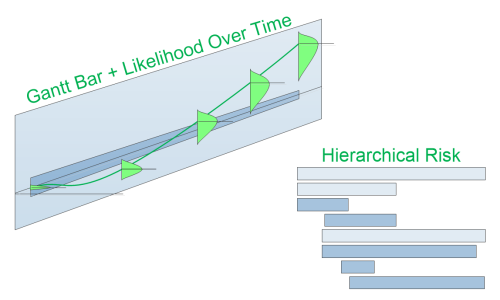
Note: In or methodology, all the time varying values from each model is represented by a single bar on a Gantt chart - so, in calculating aggregates - models/second corresponds to Bars/sec.
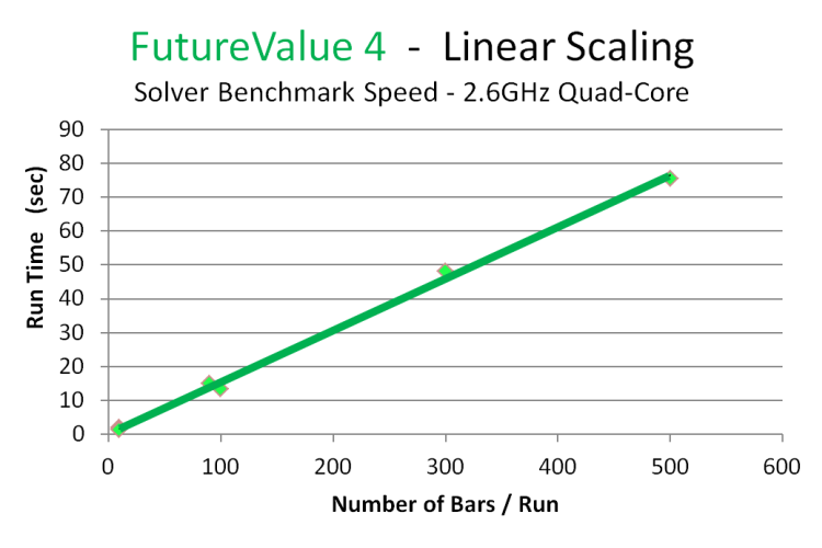
Our method scales linearly.
So, calculating aggregate Risk-Reward portfolios on a quad core laptop:
Call it roughly 400
Bars /minute with linear scaling.
We're moving the solver to a 24 core server with more memory - which should
bring the solve time for 500
Bars (independent sources of variability - varying in time) down to
about 9.5 seconds - 1000
Bars to about 19 seconds - 10,000
Bars to about 3.2 minutes (may have to add more memory for that one
- maybe not).
So, we're fast, and effectively unlimited.
Which is why we currently have 2
Patents issued and 7
Patents pending.